Data-reading module diag_rb in the post-processing program diag ¶

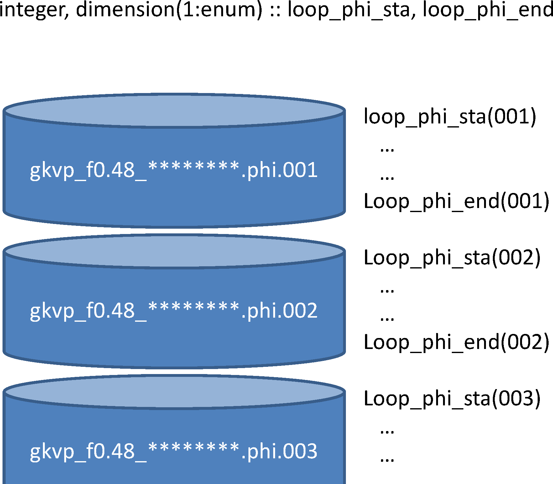
../../_images/output_record.png — Fig. 1 Output record number in the post-processing program `diag` ¶

To read GKV binary output in the post-processing program diag , use the data-reading module diag_rb .

          
           Listing 1
          
           An example to use diag_rb
          
           ¶
          
           use diag_rb, only : rb_phi_loop
complex(kind=DP) :: phi(-nx:nx, 0:global_ny, -global_nz:global_nz-1)
integer :: loop = 100
call rb_phi_loop(loop, phi) ! Read potential phi at output record loop=100 (time=dtout_ptn*loop)

The output record number loop is counted up from the first run ( inum =1) by evaluating file size of GKV binary output. As shown in Fig. 1 , output record number for the binary output $DIR/phi/*phi* is from loop_phi_sta (001) = 0 to loop_phi_end(enum) = nloop_phi . Therefore, even if you analyze only run numbers from snum $>1$ to enum , all GKV binary output data from inum =1 should be left in the diagnosed directory.

Taking a look at the source code of diag_rb , one finds various types of subroutines which read electrostatic potential $\tilde{\phi}_{\bm{k}}$ in $(k_x,k_y,z)$ or in $(k_x,k_y)$ at a given $z$ or in $(z)$ for a given mode $k_x, k_y$ , etc., and similarly read magnetic vector potential $\tilde{A}_{\parallel\bm{k}}$ , fluid moments, and so on. Some typical subroutines are listed below. One may find more efficient subroutine in the source code of diag_rb .

List of subroutines in the data-reading module diag_rb

Table 23 rb_phi_gettime(loop, time) ¶
Field	Description
Arguments	integer, intent(in) :: loop real(kind=DP), intent(out) :: time
GKV binary output	phi/gkvp_f0.48_(rankg in 6 digits).0.phi.(inum in 3 digits)
Description	Read simulation time $time$ corresponding to the output record $loop$ . ( $time \simeq dtout\_ptn \times loop$ )

Table 24 rb_Al_gettime(loop, time) ¶
Field	Description
Arguments	integer, intent(in) :: loop real(kind=DP), intent(out) :: time
GKV binary output	phi/gkvp_f0.48_(rankg in 6 digits).0.Al.(inum in 3 digits)
Description	Read simulation time $time$ corresponding to the output record $loop$ . ( $time \simeq dtout\_ptn \times loop$ )

Table 25 rb_mom_gettime(loop, time) ¶
Field	Description
Arguments	integer, intent(in) :: loop real(kind=DP), intent(out) :: time
GKV binary output	phi/gkvp_f0.48_(rankg in 6 digits).(ranks in 1 digit).mom.(inum in 3 digits)
Description	Read simulation time $time$ corresponding to the output record $loop$ . ( $time \simeq dtout\_ptn \times loop$ )

Table 26 rb_trn_gettime(loop, time) ¶
Field	Description
Arguments	integer, intent(in) :: loop real(kind=DP), intent(out) :: time
GKV binary output	phi/gkvp_f0.48_(rankg in 6 digits).(ranks in 1 digit).trn.(inum in 3 digits)
Description	Read simulation time $time$ corresponding to the output record $loop$ . ( $time \simeq dtout\_eng \times loop$ )

Table 27 rb_phi_loop(loop, phi) ¶
Field	Description
Arguments	integer, intent(in) :: loop complex(kind=DP), intent(out) :: phi(-nx:nx,0:global_ny,-global_nz:global_nz-1)
GKV binary output	phi/gkvp_f0.48_(rankg in 6 digits).0.phi.(inum in 3 digits)
Description	Read electrostatic potential $phi$ corresponding to the output record $loop$ . ( $time \simeq dtout\_ptn \times loop$ )

Table 28 rb_Al_loop(loop, Al) ¶
Field	Description
Arguments	integer, intent(in) :: loop complex(kind=DP), intent(out) :: Al(-nx:nx,0:global_ny,-global_nz:global_nz-1)
GKV binary output	phi/gkvp_f0.48_(rankg in 6 digits).0.Al.(inum in 3 digits)
Description	Read vector potential $Al$ corresponding to the output record $loop$ . ( $time \simeq dtout_ptn \times loop$ )

Table 29 rb_mom_imomisloop(imom, is, loop, mom) ¶
Field	Description
Arguments	integer, intent(in) :: imom, is, loop complex(kind=DP), intent(out) :: mom(-nx:nx,0:global_ny,-global_nz:global_nz-1)
GKV binary output	phi/gkvp_f0.48_(rankg in 6 digits).(ranks in 1 digit).mom.(inum in 3 digits)
Description	Read a fluid moment $mom$ corresponding to the output record $loop$ ( $time \simeq dtout\_ptn * loop$ ), where $is$ specifies the plasma species, and $imom=0-5$ correspond to $\tilde{n}_{\mathrm{s}\bm{k}}$ , $\tilde{u}_{\parallel\mathrm{s}\bm{k}}$ , $\tilde{p}_{\parallel\mathrm{s}\bm{k}}$ , $\tilde{p}_{\perp\mathrm{s}\bm{k}}$ , $\tilde{q}_{\parallel\parallel\mathrm{s}\bm{k}}$ , $\tilde{q}_{\parallel\perp\mathrm{s}\bm{k}}$ .

Table 30 rb_trn_itrnisloop(itrn, is, loop, trn) ¶
Field	Description
Arguments	integer, intent(in) :: itrn, is, loop real(kind=DP), intent(out) :: trn(-nx:nx,0:global_ny)
GKV binary output	phi/gkvp_f0.48_(rankg in 6 digits).(ranks in 1 digit).trn.(inum in 3 digits)
Description	Read a variable corresponding to the entropy balance $trn$ at the output record $loop$ ( $time \simeq dtout\_eng * loop$ ), where $is$ specifies the plasma species, and $itrn=0-11$ correspond to perturbed gyrocenter entropy, electrostatic field energy including polarization, magnetic field energy, wave-particle interaction via electrostatic fluctuations, wave-particle interaction via magnetic fluctuations, nonlinear entropy transfer via $\bm{E}\times\bm{B}$ flows, nonlinear entropy transfer via magnetic flutters, collisional dissipation, particle flux by $\bm{E}\times\bm{B}$ flows, particle flux by magnetic flutters, energy flux by $\bm{E}\times\bm{B}$ flows, energy flux by magnetic flutters.