3. Discretization 
3.1. Spatial discretization 
GKV is a Vlasov (continuum) simulation code. The perpendicular directions are already given by a discrete representation in Fourier space \((k_x, k_y)\) . The other three directions \((z,v_\parallel,\mu)\) are discretized by an equidistant grid. Defining box sizes \(-L_x \leq \bar{x} < L_x, -L_y \leq \bar{y} < L_y, -L_z \leq \bar{z} < L_z, -L_v \leq \bar{v}_\parallel \leq L_v, 0 \leq \bar{\mu} \leq \frac{L_v^2}{2}\) and grid numbers \((2\mathtt{nx}+1,\mathtt{global\_ny}+1,2\mathtt{global\_nz},2\mathtt{global\_nv},\mathtt{global\_nm}+1)\) in \((k_x,k_y,z,v_\parallel,\mu)\) , the grid of GKV is given by
where \(\Delta k_x = \frac{\pi}{L_x}, \Delta k_y = \frac{\pi}{L_y}, \Delta z = \frac{L_z}{\mathtt{global\_nz}}, \Delta v_\parallel = \frac{2L_v}{2\mathtt{global\_nv}-1}, \Delta w = \frac{L_v}{\mathtt{global\_nm}}\) .
Derivatives in \((z,v_\parallel,\mu)\) are discretized by finite difference method, and then, GKV solves the \(\delta f\) gyrokinetic equations, Eqs. (2.2) – (2.4) , in \((k_x,k_y,z,v_\parallel,\mu)\) space, except for the nonlinear term. Since direct calculation of nonlinear convolution in wavenumber space is computationally expensive, the nonlinear term is evaluated in the real space, employing \((2\mathtt{nxw},2\mathtt{nyw},2\mathtt{global\_nz},2\mathtt{global\_nv},\mathtt{global\_nm}+1)\) grid points in \((x,y,z,v_\parallel,\mu)\) , and is transformed back to the wavenumber space by means of 2D Fast Fourier Transform (FFT) algorithm and the 3/2 de-aliasing rule in \((k_x, k_y)\) .
To implement the pseudo-periodic boundary condition along a field line,
Eq.
(1.16)
, the shift of the radial wave number
\(\delta k_x (k_y) = - 2N_\theta \pi \hat{s} k_y\)
as a function of
\(k_y\)
should be equal to the integral multiple of the minimum radial wave
number
\(\Delta k_x\)
. This gives a constraint between radial and
field-line-label box sizes. In GKV, the minimum field-line-label wave
number
\(\Delta k_y\)
and the ratio
\(m = \left| \frac{\delta k_x (\Delta k_y)}{N_\theta \Delta k_x} \right|\)
are given in the namelist (
kymin
and
m_j
, respectively), and then,
\(\Delta k_x = |2\pi \hat{s} \Delta k_y / m|\)
,
\(L_x = \pi /\Delta k_x\)
,
\(L_y = \pi / \Delta k_y\)
.
3.1.1. Choice of velocity-space coordinate 
After gkvp_f0.63, altanate velocity space coordinate, the parallel and perpendicular velocities \((v_\parallel, v_\perp)\) rather than the magnetic coordinate \((v_\parallel, \mu)\) . This choice is beneficial when the magnetic field strength significantly varies, like the dipole geometry. Switching the velocity-space coordinates is done in run/gkvp_namelist:
vp_coord = 0, # For (vl,mu) coordinates
or
vp_coord = 1, # For (vl,vp) coordinates
In the equation, the parallel advection term is modified:
3.2. Temporal discretization 
3.2.1. Explicit implementation 
GKV usually uses 4th-order explicit Runge-Kutta-Gill method. [ 3-1 ]
3.2.2. Explicit collisionless physics and implicit collision implementation 
An alternative option is implicit collision solver which is useful for Lorentz or Sugama collision operators having velocity-dependent collision frequencies [ 3-2 ] . Splitting collisionless physics and collision operator by means of 2nd-order (Strang) operator split, the collisionless physics is solved by using 4th-order explicit Runge-Kutta-Gill method, while the collision operator is solved by using 2nd-order semi-implicit Crank-Nicolson method. Bi-CGSTAB method is used as an iterative matrix solver for implicit collision.
3.3. Inter-node decomposition by using MPI 
The computations are parallelized by using the OpenMP/MPI hybrid parallelization which suites for hierarchical hardware of the nodes having a number of cores with a shared memory and connected by an interconnect network.
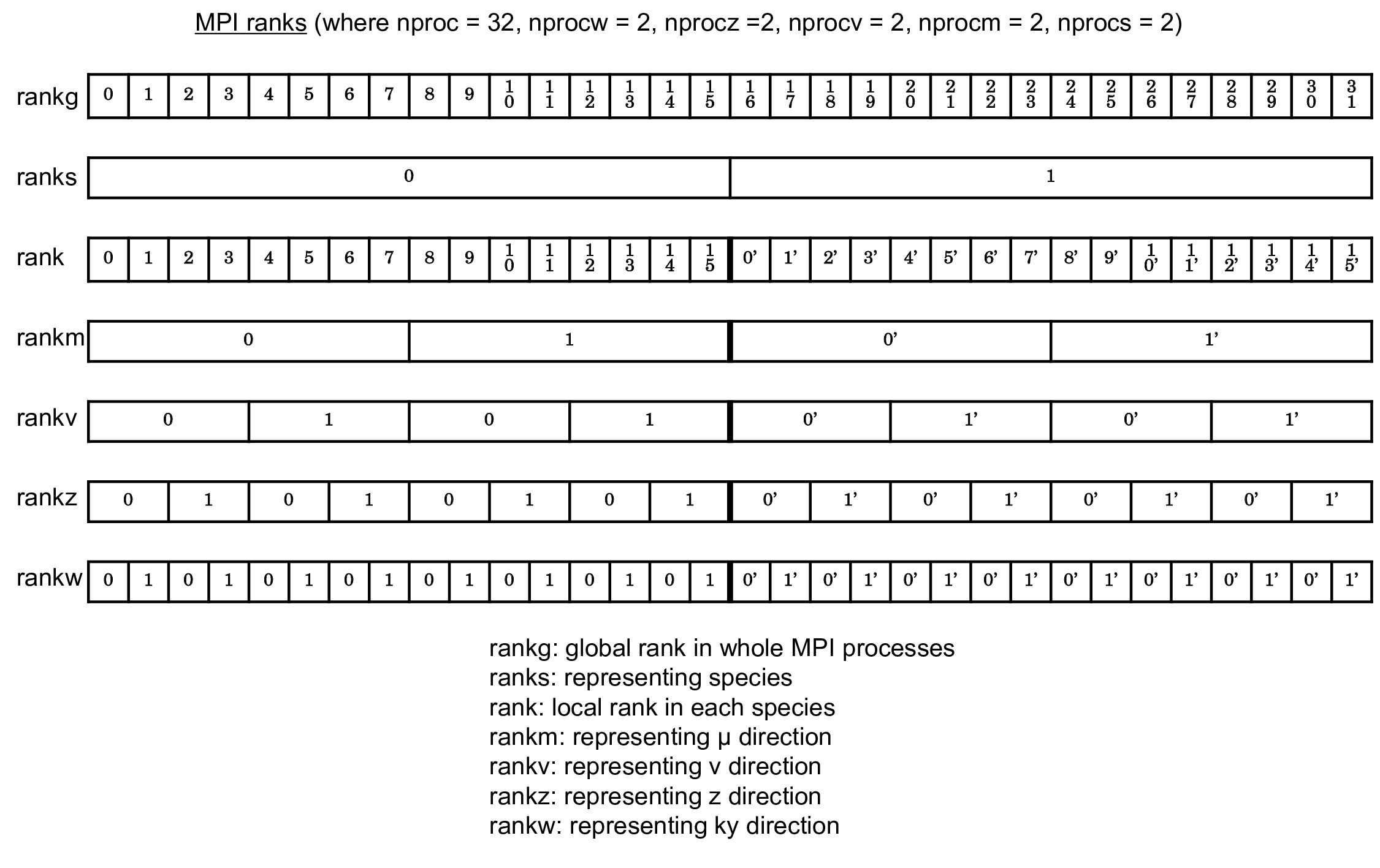
Fig. 3.1 An example of MPI ranks in GKV. 
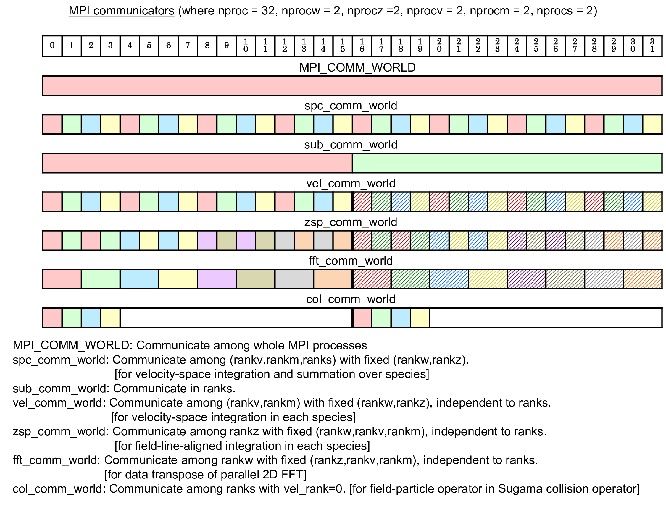
Fig. 3.2 An example of MPI communicators in GKV. 
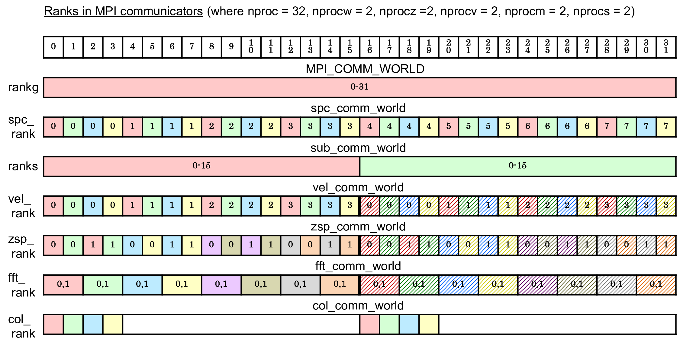
Fig. 3.3 An example of MPI ranks in communicators in GKV. 
Taking advantage of the multi-dimensional problem, multi-dimensional
domain decomposition is applied for
\(y\)
,
\(z\)
,
\(v_\parallel\)
,
\(\mu\)
and
\(s\)
, where 2D FFTs in
\(x\)
and
\(y\)
are parallelized by means of the
transpose split method. Then, the required MPI communications are data
transpose for the parallel 2D FFTs in
\(x\)
and
\(y\)
, point-to-point
communications in
\(z\)
,
\(v_\parallel\)
and
\(\mu\)
for finite difference
methods, and reduction communications over
\(v_\parallel\)
,
\(\mu\)
and
\(s\)
for velocity-space and species integration.
Figures
3.1
–
3.3
show schematic pictures of
the multi-layer structure of the multi-dimensional domain decomposition,
illustrating the case that
\(y\)
,
\(z\)
,
\(v_\parallel\)
,
\(\mu\)
and
\(s\)
are
respectively split by two MPI processes (and thus
\(2^5=32\)
processes in
total). Plasma species
\(s\)
are decomposed as
\(\texttt{ranks} = 0, 1\)
,
and each species are hierarchically decomposed by the magnetic moment
\(\mu\)
(
rankm
), the parallel velocity
\(v_\parallel\)
(
rankv
), the
parallel direction
\(z\)
(
rankz
), and the perpendicular direction
\(x,y\)
(
rankw
). Thus, data transpose in
\(x\)
and
\(y\)
is performed for
different subranks of
rankw
by using
fft_comm_world
communicator,
point-to-point communications in
\(z\)
(
\(v\)
or
\(m\)
) are performed between
rankz
(
rankv
or
rankm
), while reduction communications over
\(v\)
,
\(\mu\)
and
\(s\)
are performed for fixed
rankz
and
rankw
by using
spc_comm_world
communicator.
3.4. Intra-node decomposition by using OpenMP 
Intra-node decomposition is basically implemented by loop-level parallelization with OpenMP. Time-consuming MPI communications are masked by computation-communication overlap technique using MASTER thread. For more details, see Ref. [ 3-3 ] .
S. Gill. A process for the step-by-step integration of differential equations in an automatic digital computing machine. Proc. Cambridge Philosophical Soc. , 47(1):96–108, 1951. doi:10.1017/S0305004100026414 .
S. Maeyama, T.-H. Watanabe, Y. Idomura, M. Nakata, and M. Nunami. Implementation of a gyrokinetic collision operator with an implicit time integration scheme and its computational performance. Comput. Phys. Commun. , 235:9–15, 2019. doi:https://doi.org/10.1016/j.cpc.2018.07.015 .
S. Maeyama, T.-H. Watanabe, Y. Idomura, M. Nakata, M. Nunami, and A. Ishizawa. Improved strong scaling of a spectral/finite difference gyrokinetic code for multi-scale plasma turbulence. Parallel Comput. , 49:1–12, 2015. doi:https://doi.org/10.1016/j.parco.2015.06.001 .